A Guide to Machine Learning Optimization Techniques for Smarter Models

Imagine you’ve built a machine learning model to analyze customer behavior and boost sales for your business. The model is accurate and delivers excellent results. But what if you could make it even smarter, faster, and more efficient? That’s the goal of machine learning optimization. By optimizing your model, you can reduce its computational cost and improve its performance. In this article, we’ll explore machine learning optimization: why it matters and how to achieve it. Doing so will help you build better machine learning models that deliver high performance with minimal computational cost.

One of the best ways to optimize machine learning models is by using AI inference APIs, like those offered by Inference. These tools can help your business achieve its objectives by streamlining machine learning model operations to make them more efficient.

What Does Optimization Mean in Machine Learning?

Optimization is adjusting a machine learning model's parameters to minimize errors and improve performance. To illustrate the concept, consider linear regression. Linear regression makes predictions by calculating the weighted average of input features to arrive at an output.

The outcome is linear: It assumes a straight-line relationship between variables.

Optimization in linear regression aims to determine the best weights for the model. An optimization algorithm minimizes a loss function, which measures the gap between the predicted and actual values in the training data. In doing so, the algorithm improves the accuracy of the model’s predictions. The better the model makes these predictions on the training data, the more accurate it will be at predicting values for new data.

Understanding Optimization Algorithms

In machine learning, optimization refers to finding a model's best parameters. This process is achieved through various optimization algorithms that update model parameters during training.

Algorithms differ by how they search for the best parameters and can be broadly categorized into two groups:

• Deterministic: Deterministic algorithms, like gradient descent, use the entire dataset to calculate the loss function and derive the optimal weights.
• Stochastic: Unlike genetic algorithms, stochastic algorithms use a random dataset sample to make calculations. They are more exploratory and can help avoid local minima that deterministic methods may reach.

Why Optimization Matters

Optimization is integral to machine learning. Model training relies on improving accuracy and reducing errors, which is an optimization problem. For example, a data scientist provides labeled training data when training a model.

The model makes predictions about the data, improving its accuracy through optimization with each iteration. Accurate predictions about the training data will help the model perform better on new data.

Optimization and Hyperparameters

When we talk about hyperparameter optimization in machine learning, we refer to the process of tuning a model's configurations to improve performance. Hyperparameters are distinct from model parameters. They are set before the training process and control how a model learns.

Unlike parameters, which are automatically optimized, data scientists must tune hyperparameters manually. The learning rate, number of hidden layers, and the number of clusters in a classification task are all examples of hyperparameters.

Why Hyperparameter Optimization is Important

Hyperparameter optimization is essential for creating accurate machine learning models. The process can be difficult. Selecting the wrong hyperparameters can lead to inaccurate models that either underfit or overfit training data. Underfitting occurs when a model is improperly trained and cannot accurately predict the training set or new data.

Overfitting happens when a model learns the training data too well, capturing noise, outliers, and underlying patterns. Such a model will perform well on the training data but will be inaccurate when predicting new data. Hyperparameter optimization aims to improve a model’s performance on training and unseen datasets.

Related Reading

• How to Improve Machine Learning Models
• LLM Inference Optimization
• Real-time Machine Learning

An Overview of Machine Learning Optimization Techniques

Parameters and hyperparameters are vital components of machine learning models. Parameters are the variables the model uses to make its predictions. Hyperparameters, on the other hand, are the settings for the model that must be configured before training. To understand the difference between these two notions, let’s break them down further. The model “learns” the parameters during training. You can think of them as the internal variables of the model that change based on the input data. For example, in a neural network, these include the weights and biases of the various nodes.

Optimizing Hyperparameters for Better Model Accuracy

Hyperparameters are “not learned” by the machine but are instead set before training begins. They help to configure the model and determine its structure. For instance, they include the number of clusters in a clustering model, the learning rate, and the number of layers in a neural network. Tuning hyperparameters is crucial for improving model accuracy and performance. Since they influence how the model learns the parameters, optimizing their values can significantly reduce error and enhance the machine learning model's predictive capabilities.

Understanding Hyperparameter Tuning

As we said, the hyperparameters are set before training. But you can’t know in advance, for instance, which learning rate (large or small) is best in this or that case. To improve the model’s performance, hyperparameters have to be optimized. After each iteration, you compare the output with expected results, assess the accuracy, and adjust the hyperparameters if necessary. This is a repeated process. You can do that manually or use one of the many optimization techniques that come in handy when working with large amounts of data.

Comparing Optimization Techniques in Machine Learning

Now, let us talk about the techniques you can use to optimize the hyperparameters of your model.

Exhaustive Search

An exhaustive or brute-force search looks for the most optimal hyperparameters by checking whether each candidate is a good match. You perform the same thing when you forget the code for your bike’s lock and try all the possible options. We do the same thing in machine learning, but the number of options is quite large. The exhaustive search method is simple. For example, if you work with a k-means algorithm, you will manually search for the correct number of clusters. If there are hundreds and thousands of options that I have to consider, it becomes unbearably heavy and slow. This makes brute-force search inefficient in most real-life cases.

Gradient-Based Optimization Techniques

Gradient descent is the most common algorithm for optimizing models to minimize errors. To perform gradient descent, you iterate over the training dataset while re-adjusting the model.

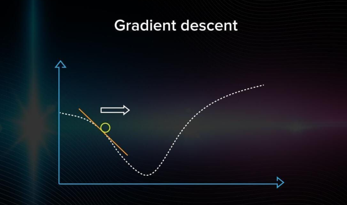
You aim to minimize the cost function because doing so ensures the fewest possible errors and improves the model's accuracy.

The graph shows a graphical representation of how the gradient descent algorithm travels in the variable space. You must take a random point on the graph and arbitrarily choose a direction. If you see that the error is getting larger, that means you chose the wrong direction.

The Impact of Learning Rate on Gradient Descent

When you can no longer improve (decrease the error), the optimization is over, and you have found a local minimum.

Note: In gradient descent, you proceed with steps of the same size. If you choose a learning rate that is too large, the algorithm will jump around without getting closer to the right answer. If it’s too small, the computation will start mimicking an exhaustive search, which is inefficient.

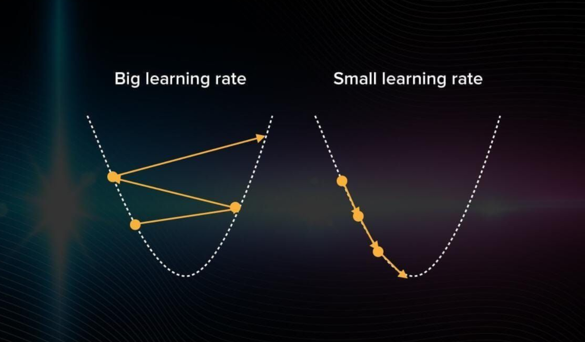
You have to choose the learning rate very carefully. If done right, gradient descent becomes a computation-efficient and quick method of optimizing models. 

Stochastic Gradient Descent with Momentum

Stochastic Gradient Descent (SGD) is an optimization algorithm used in machine learning and deep learning for training models. It is an extension of the standard gradient descent algorithm, where instead of computing the gradient of the entire dataset, SGD computes the gradient and updates the model parameters for each training example individually or in small batches. Why use SGD:

• Computational Efficiency: Computing the gradient using the entire dataset can be computationally expensive, especially for large datasets. SGD allows for more frequent updates with lower computational cost.
• Faster Convergence: Since updates are made more frequently, SGD converges faster than traditional gradient descent, especially when dealing with non-convex loss functions.
• Memory Efficiency: Working with individual or mini-batches of data requires less memory than the entire dataset, making SGD suitable for cases where memory is a constraint.
• Escape Local Minima: SGD's stochastic nature introduces randomness into the optimization process, helping the algorithm escape local minima and explore the parameter space more effectively.

It’s an extension of gradient descent where the parameters are updated using a single randomly chosen data point at a time, making it computationally less expensive. The disadvantage of this method is that it requires a lot of updates, and the steps of gradient descent are noisy. Because of this, the gradient can go in the wrong direction and become very computationally expensive. That is why other optimization algorithms are often used.

RMSProp

RMSprop is an optimization algorithm designed to address some of the limitations of traditional gradient descent, especially when dealing with non-convex and poorly conditioned optimization problems. It is beneficial for problems with sparse data and helps to adjust the learning rates for different parameters adaptively. How RMSprop Works:

RMSprop adapts the learning rates of each parameter individually by dividing the learning rate by the root mean square of recent gradients. This allows the algorithm to automatically decrease the learning rate for parameters with steep and rapidly changing gradients and increase the learning rate for parameters with small or slowly changing gradients.

Adam Optimizer

Adam is an optimization algorithm used for training machine learning models. It combines ideas from momentum optimization and RMSprop (Root Mean Square Propagation). Adam adapts the learning rates for each parameter individually based on their historical gradients. Why Adam?

• Adaptive Learning Rates: One of Adam's key advantages is its adaptive learning rate mechanism. It adjusts the learning rates for each parameter based on the historical gradients, allowing it to perform well across different parameters and features.
• Efficiency in Sparse Gradients: Adam is well-suited for sparse gradients, which are common in tasks like natural language processing. It maintains a separate adaptive learning rate for each parameter, making it less sensitive to the scale of the gradients.
• Combining Momentum and RMSprop: Adam combines the momentum term to accelerate convergence in the parameter space with the RMSprop term to scale the learning rates adaptively. This combination helps handle noisy gradients and navigate through saddle points efficiently.
• Effective in a Wide Range of Applications: Adam has shown effectiveness in a wide range of deep learning applications and is widely used in practice due to its robust performance and ease of use.

Gradient-Free Optimization Techniques

Genetic algorithms represent another approach to ML optimization. The logic behind these algorithms attempts to apply the theory of evolution to machine learning. In the theory of evolution, only those specimens get to survive and reproduce that have the best adaptation mechanisms. How do you know what specimens are and aren’t the best in the case of machine learning models?

Understanding Genetic Algorithms in Model Selection

Imagine you have a bunch of random algorithms at hand. This will be your population. Among multiple models with some predefined hyperparameters, some are better adjusted than the others. Let’s find them!

• You calculate the accuracy of each model.
• You keep only those that worked out best.
• Now, you can generate some descendants with hyperparameters similar to the best models to get a second generation of models.

You can see the logic behind this algorithm in this picture:

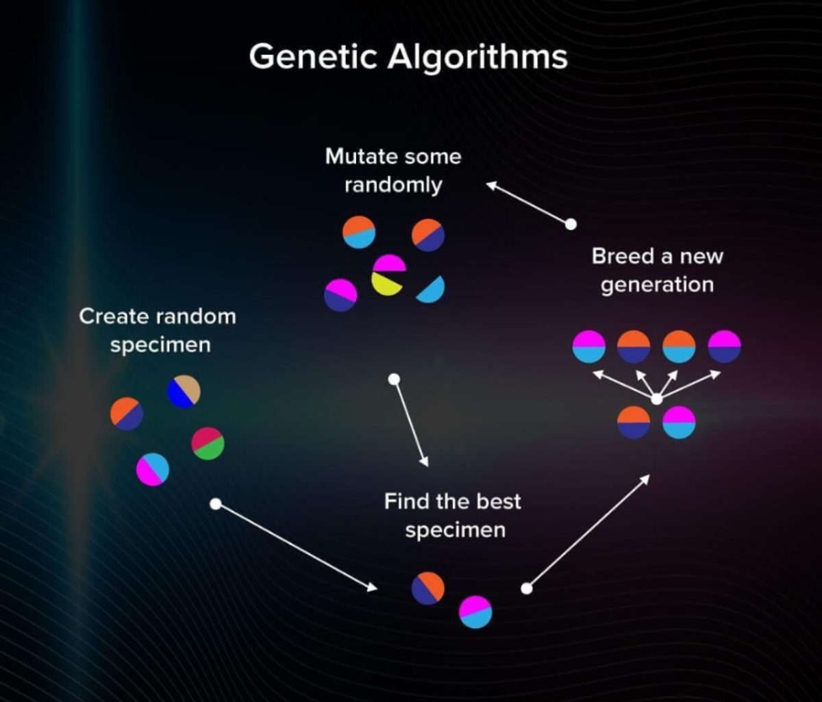
We repeat this process many times, and only the best models will survive. Genetic algorithms help to avoid being stuck at local minima/maxima. They are common in optimizing neural network models. 

Exhaustive Search

Pros

• All possible options are evaluated.
• The most intuitive one.

Cons

• When there are many solutions, it becomes extremely slow.

Where to Use

• The database is small.
• High accuracy is more important than the cost and speed of computation.

Gradient

Pros

• Computationally efficient.
• Stable.
• Easy and quick to use.

Cons

• Doesn't work if there are multiple local minima.
• You risk skipping the right solution if the learning rate is too large.

Where to Use

• Need to optimize the model fast.
• You can’t calculate the parameters linearly and have to search for them.

Genetic

Pros

• Can find good solutions in a short computation time.
• Wide range of solutions (since it’s random).

Cons

• Can’t guarantee that the solution is optimal.
• Hard to come up with good heuristics.

Where to Use

• Need to avoid getting stuck in local minima.

Random Searches and Grid Searches

Random and grid searches are the most straightforward approaches to hyperparameter machine learning optimization. A different point in a grid represents each hyperparameter configuration. Optimization involves searching these dimensions to identify the most effective hyperparameter configurations.

The process and utility of random searches and grid searches differ. Random searches are used to discover new and effective combinations of hyperparameters, as the sample is randomised. Grid searches are used to assess known hyperparameter values and combinations, as each point in the grid is searched and evaluated.

Balancing Exploration and Evaluation in Model Optimization

Random searches randomly sample different points or hyperparameter configurations in the grid. This helps to identify new combinations of hyperparameter values for the most effective model. The developer will set the number of iterations to be searched to limit the number of hyperparameter combinations. Otherwise, the process can take a long time without being limited. Grid searches as an approach often used to evaluate known hyperparameter values. Different hyperparameter values are plotted as dimensions on a grid. Whereas random searches are usually used to discover new configuration optimizations, grid searches assess the effectiveness of known hyperparameter combinations.

Evolutionary Optimization

Evolutionary optimization algorithms optimize models by mimicking the selection process within the natural world, such as the process of natural selection or genetics. Each iteration of a hyperparameter value is assessed and combined with other high-scoring hyperparameter values to form the next iteration. Hyperparameter values will be altered each interaction as a ‘mutation’ before recombining the most effective choices. Each iteration improves and becomes more effective through each ‘generation’, as it is optimized. Other approaches within evolutionary optimization include genetic algorithms. In this process, different hyperparameters are paired up after being scored as the most valuable or practical. The process continues using the resulting configuration within the next generation of tests and evaluations. Evolutionary optimization techniques are often used to train neural networks or artificial intelligence models.

Bayesian Optimization

Bayesian optimization is an iterative approach to machine learning optimization. Instead of mapping all known hyperparameter configurations on a grid as in random searches and grid searches approach, Bayesian optimization is more focused. Analysis of hyperparameter combinations happens in sequence, with previous results informing the refinements in the next experiment.

As the model concentrates on the most valuable areas of hyperparameters, the focus on the model improves with each step. Each iteration focuses on selecting hyperparameters in light of the target functions, so the model understands which areas of the distribution will bring the most benefit. This focuses resources and time on optimizing hyperparameters to meet specific functions.

Related Reading

• Model Compression
• LLM Latency
• Inference Time
• AI Inference vs. Training

Start Building with $10 in Free API Credits Today!

Inference delivers OpenAI-compatible serverless inference APIs for top open-source LLM models, offering developers the highest performance at the lowest cost in the market. Beyond standard inference, Inference provides specialized batch processing for large-scale async AI workloads and document extraction capabilities designed explicitly for RAG applications.

Start building with $10 in free API credits and experience state-of-the-art language models that balance cost-efficiency with high performance.

Related Reading

• Latency vs. Response Time
• Artificial Intelligence Optimization